Introduction CNN in NLP: A TensorFlow implementation of Text Classification using CNN
What will see in this article:- Overview of CNN, its use in Coumputer Vision.
- How CNN applies to NLP
CNN's delivered the major breakthroughs in the area of Computer Vision (CV) ranging from Facebook's automated photo-tagging to self-driving cars. Recenly, people have also started using CNNs in various Natrual Language Processing problems. The intution of CNN is more easier to understand for the Computer Vision (CV) applications. So we start to understand its use in CV first then slowly move towards to NLP.
Basic intution of Convolution:
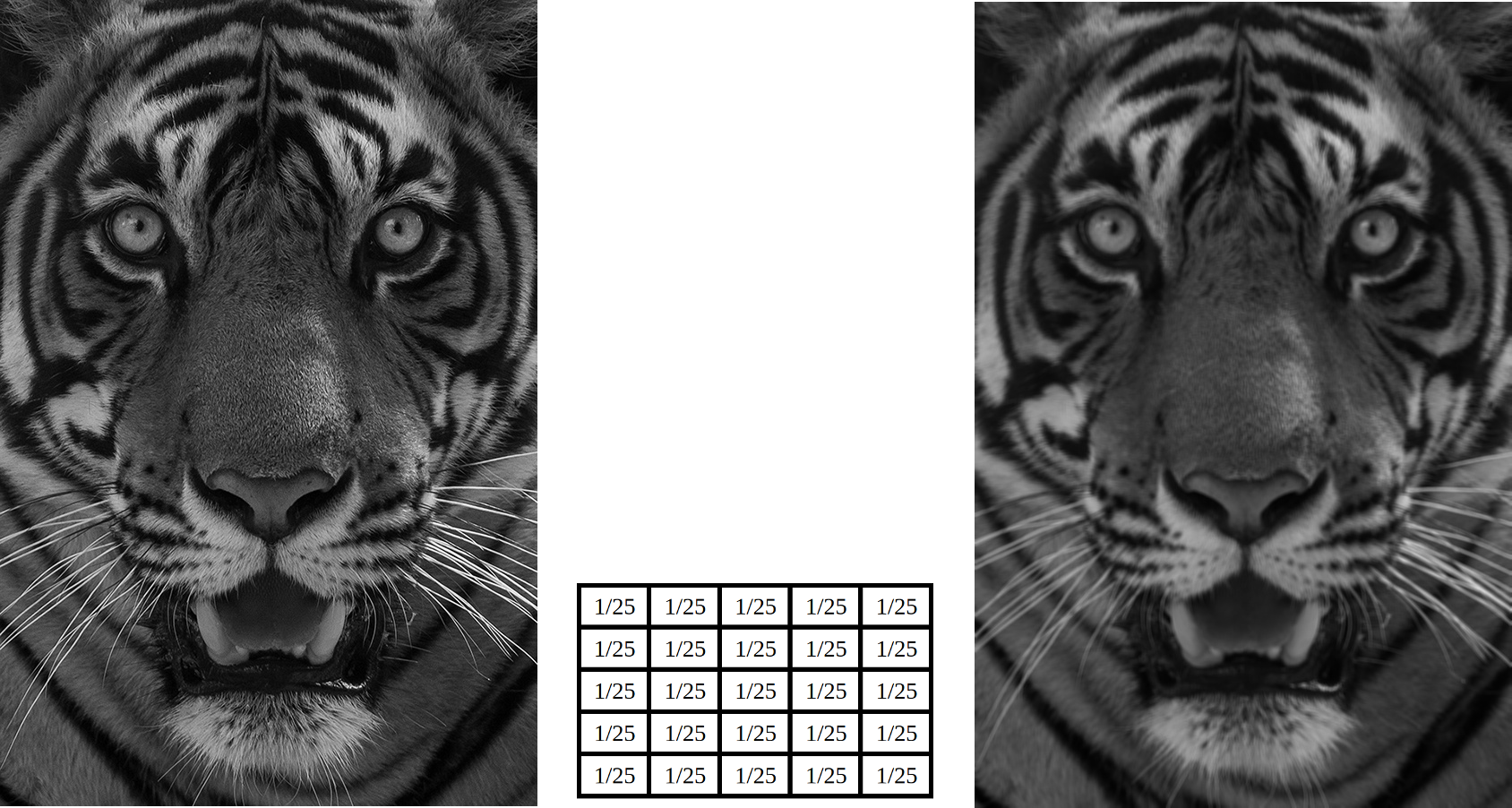
Convolution is easier to be understood by the analogy of a sliding window function applied to a matrix. Looking the figure below, it becomes quite clear:
Source: 3x3 Convolution Filter: Feature Extraction Using Convolution.
You can imagine left matrix as the image (b/w) of size 5x5, where each entry correspond to a pixel value. A sliding window of size 3x3 also called kernel, filter or feature detector is imposed on each pixel and multiply its values element-wise with origin matrix, then sum them up. This process creates convolved feature matrix of size 3x3.
There are various filters which applied in this manner in image processing. One is the averaging filter, see te figure below, which applies a 5x5 averaging filter to an image to get a smoothed picture as an output.
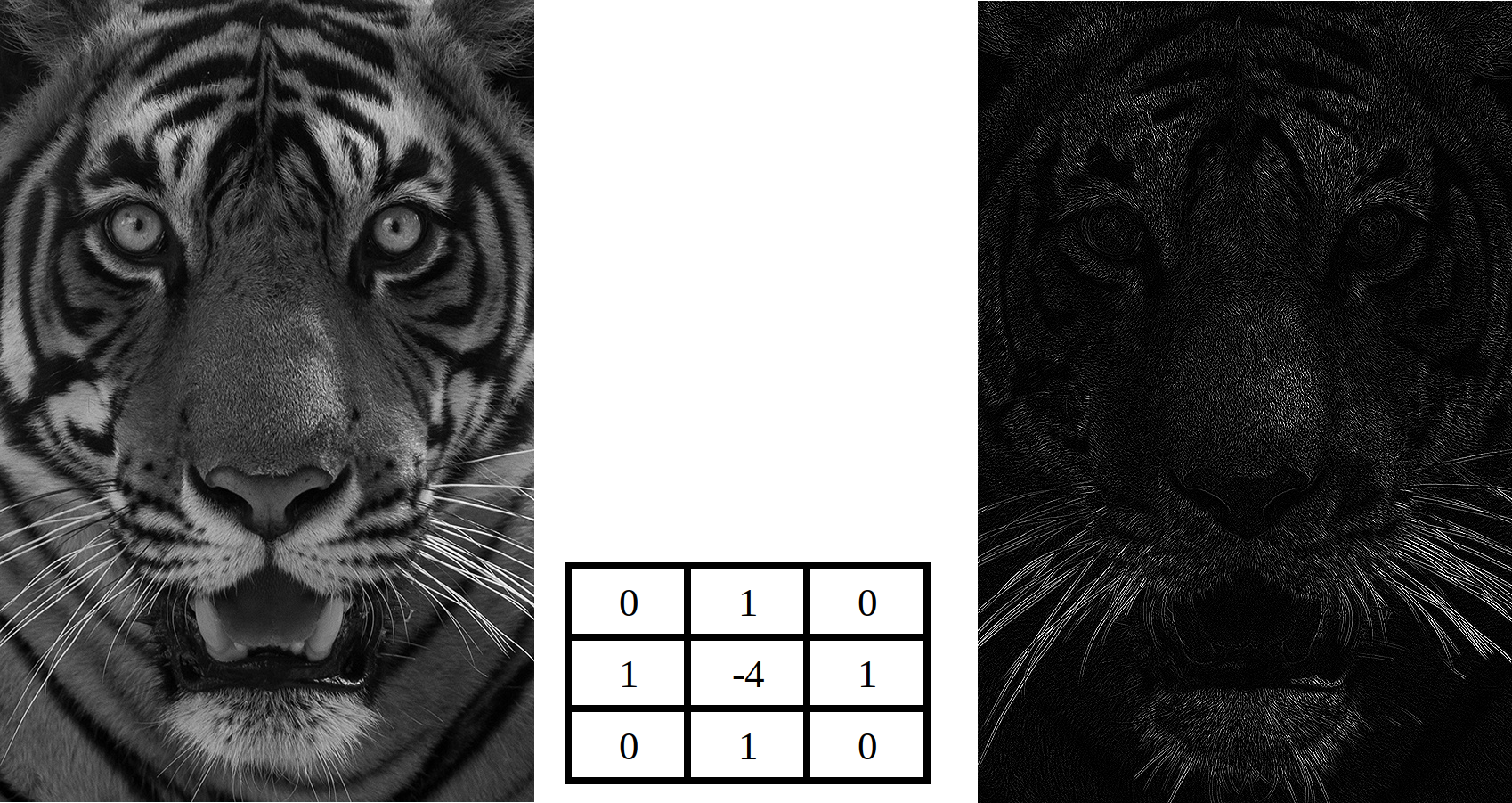
Another application of such filters is to detect edges in the image by taking the difference between a pixel and its neighbors as in example below:
Undrestanding Convolution Neural Network:
We got the intution how convolution works. But, how this concept get utilized in the CNN, is our next question. Similar to other Deep Learning models, CNN also has several leyers of convolutions with nonlinear activation functions e.g. ReLU or tanh applied to the results of each layer. In a traditional feedforward neural network, each neuron from one layer is connected to each neuron to next layer, also called as fully connected layer. But, in CNN, convolution is applied to the input to compute the output. Each layers applies different filters like the ones showed above. Pooling (subsampling) is also applied in between, we will see that later. So in the training phase, CNN automatically learns the filter values, based on the task being chosen. For example, for the image classification application, the CNN's first layer may learn to identify the edges from the input. Second layers, may use these edges to detect simples shapes in the second layer and then use these shapes to determine high-level features such as facial shapes, objects textures etc in the higher layers. The last layer use these high-level features to classify the input. See the figure below:
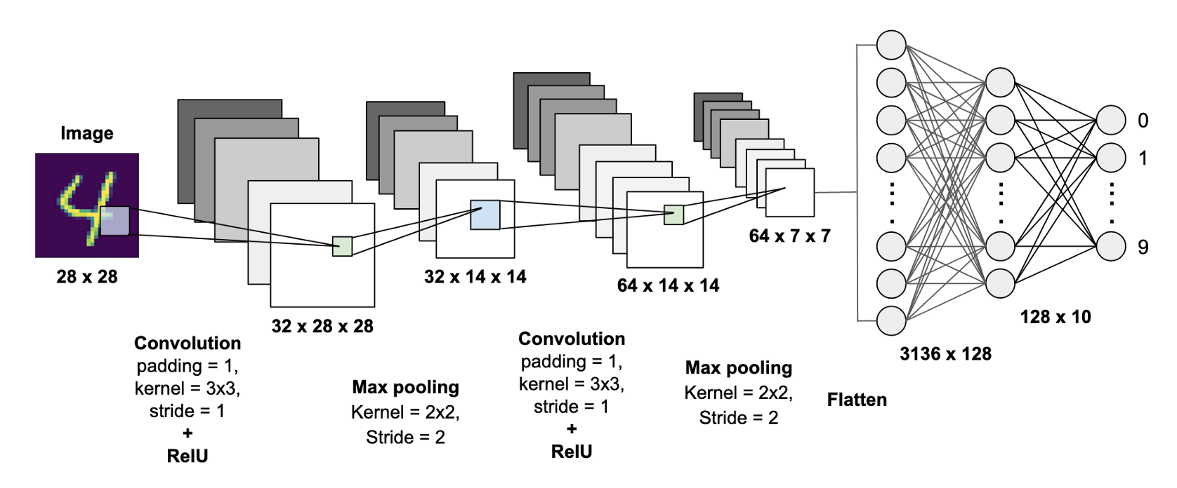
Source: MNIST Handwritten Digits Classification using a Convolutional Neural Network (CNN).
CNN is so powerful in Computer Vision due to its two inherent properties: 1. Location Invariance and Compositionality. Lets take an example of object detection in an image. Suppose, we have to detect whether elephant is there or not in the image. Pooling is invariant to translation, rotation and scaling which perform the subsampling at a layer. Second key property is compositionality which can be seen over the layers. We have seen earlier that layer-to-layers, edges are extracted from pixels, shapes are constructed from those edges and more complex objects (elephant) from shapes are build.
How CNN can be used for NLP?
Here, we have considered the Kim Yoon's work of Convolution Neural Network for a Senetence Classification as sentiment analysis. The model presented in the paper, delivers good performance over a range text classification tasks. Hence became, a standard baselines for new text classification architectures.
We taken Movie Review data from Rotten Tomatoes for the classification task. Its has total 10,662 example reviews, 50% negative and 50% positive. Its vocabulary size of approx. 20k. The preprocessing of the data is done in following steps:
- Load, negative and positive reviews separately from the raw data.
- Data is cleaned with the original pre-processing program.
-
Pad each sentence with a special token
, to the maximum sentence length of 59 for efficiently batch our data since each example in a batch must be of the same length. - Make Vocab index and map each word to its index integer between 0 to 18,758 (Vocab-Size). After this each sentence would become a vector of integers.
Implementations
This is the architecture used in the paper. First layer is the input layer which represents each word by a low-dimensional vectors. The next layer convolves the word vectors through multiple filter sizes, e.g. sliding over 3,4 or 5 words at a time. The next layer extracts the max-pool result of the convolutional layer into a long feature vector. At the last, classify the result using a softmax layer. Further, all the layers and their inner-working is discussed thoroughly.
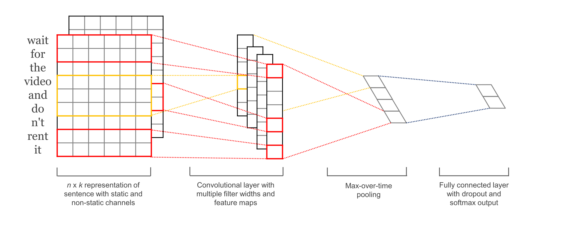
Source (paper): Convolutional Neural Networks for Sentence Classification.
CNN architecture is defined in the text_cnn.py and all other data loading, traning and development routines are defined in the train.py file. Let's define the architecture first then the traning procedure.
TextCNN class initialisation
Entire CNN configuration is defined in the TextCNN class inside the text_cnn.py program using Tensorflow.
"""
A CNN for text classification.
Uses an embedding layer, followed by a convolutional, max-pooling and softmax layer.
"""
def __init__(
    self, sequence_length, num_classes, vocab_size,
    embedding_size, filter_sizes, num_filters, l2_reg_lambda=0.0):
TextCNN class is initialized with some parameters. sequence_length defines the number of words (actual+padded) in an utterance which is 56. num_classes number of classes 2, an utterance may be assigned to. vocab_size to show the number of total possible words in the dataset that is 18,758. embedding_size decides the length of word-vector which is 128. filter_sizes is a list of number deciding each filter's size to be used during the convolution which is \[3,4,5\], means we have filters which slide over 3,4,5 words respectively. num_filters shows the number of channels the filter will generate value for. l2_reg_lambda is a regularization paramerter for L2_norm which is set to zero, means optional.
Input Placeholders
Tensorflow placeholders are defined for input_x, input_y and dropbout_keep_prob variables.
# Placeholders for input, output and dropout
self.input_x = tf.placeholder(tf.int32, [None, sequence_length], name="input_x")
self.input_y = tf.placeholder(tf.float32, [None, num_classes], name="input_y")
self.dropout_keep_prob = tf.placeholder(tf.float32, name="dropout_keep_prob")
tf.placehoder function make a placeholder variable that we feed to the network during the training and testing. The first element denotes the type of values e.g. int32, float32 etc, would be assigned to the variable, second the shape of the variable where 'None' tells that the dimensions will decided at the run time. In our case, it is equal to batch-size=64, name="some_name" is the name of that variable. dropout_keep_prob tells how many nerons will not be passed to the next layer. Its value is 0.5, means 50% of the values will be set to zero before transmittting to the next layer.
Embedding Layer
Just to understand how CNN works for the simple sentence-classification, we have simplified some of the operations. We are not using pre-trained word2vec to represent word-embeddings. Instead, we learn it from the scratch (see below code snippet). self.W tensor is created of size vocab_size=18,758 and embedding_size=128, from which the desired word-embeddings will be looked upon. We have considered only one non-static word vectors as input channel for word-embeddings.
# Embedding layer
with tf.device('/cpu:0'), tf.name_scope("embedding"):
    self.W = tf.Variable(
        tf.random_uniform([vocab_size, embedding_size], -1.0, 1.0),
        name="W")
    self.embedded_chars = tf.nn.embedding_lookup(self.W, self.input_x)
    self.embedded_chars_expanded = tf.expand_dims(self.embedded_chars, -1)
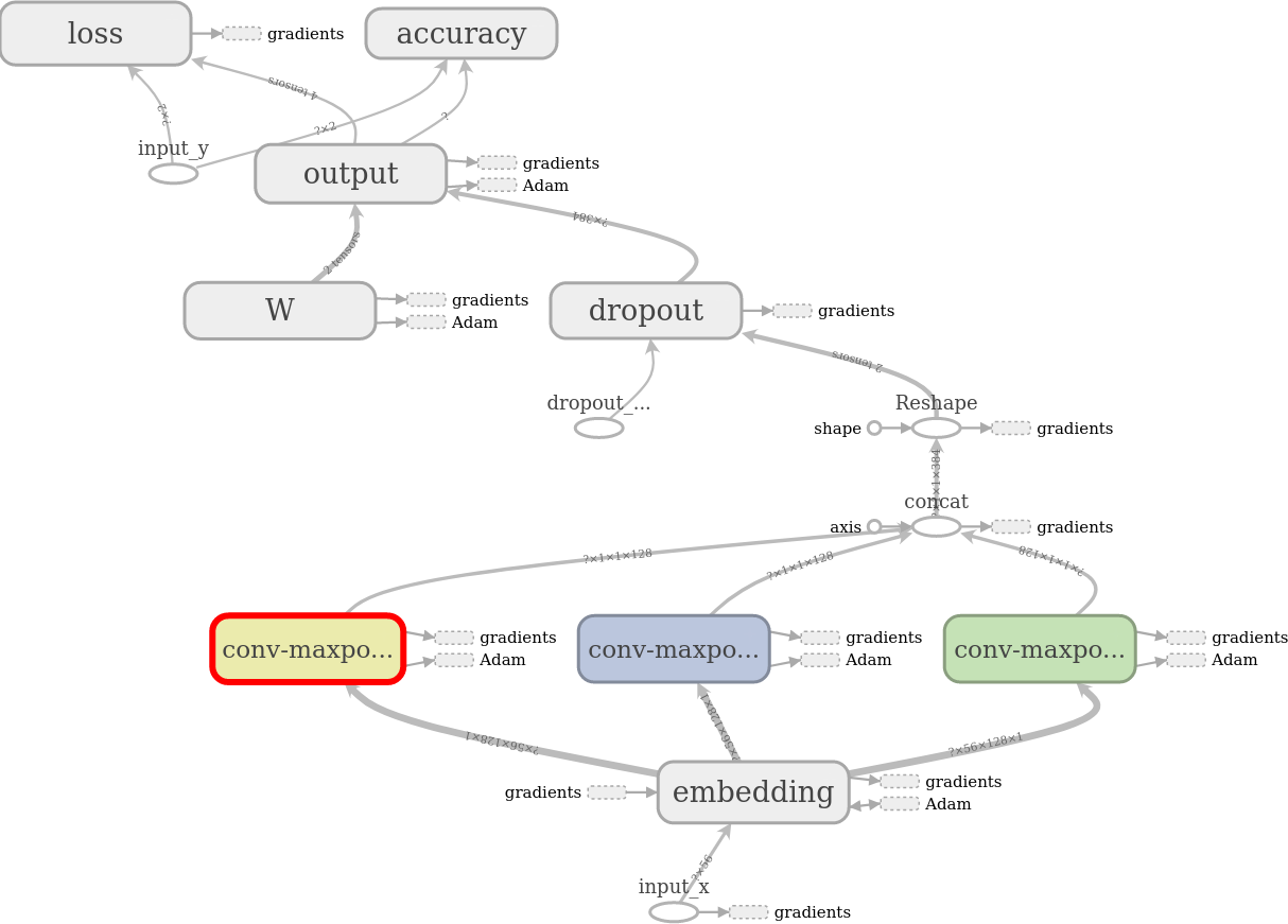
tf.device("/cpu:0") forces the operations to be excecuted on the CPU only. tf.name_scope("embedding") assigns this name to the node, visible as a nice hierarchy when visualizing the network in TensorBoard by executing command "tensorboard --logdir runs/1583250809/summaries/" on the shell.
'W' is the embedding matrix which we learn during the training which is initialised using a random_uniform distribution. tf.nn.embedding_lookup helps in looking-up a embedding from an input-word. The result of this operation has shape \[None(batch_size=64), sequence_length(56), embedding_size(128)\]. The convolution (Conv2d) layers require input to of 4 dimension \[batch(64), width(56), height(128), channel(1)\]. Hence, we use tf.expand_dims to expand 1 more dimension representing the channel.
Convolution and Max-Pooling Layers
Here, we have decided to use three convolutional-layers of different filter_sizes which decides the number words the filters slide-over. The chosen filter-sizes are 3,4 and 5. Each layer will will take embeddings as input independently and generate tensors of different shapes. The results of all the convolution-layer will be concatenated into a big feature-vector as described in the code.
# Create a convolution + maxpool layer for each filter size
pooled_outputs = []
for i, filter_size in enumerate(filter_sizes):
    with tf.name_scope("conv-maxpool-%s" % filter_size):
        # Convolution Layer
        filter_shape = [filter_size, embedding_size, 1, num_filters]
        W = tf.Variable(tf.truncated_normal(filter_shape, stddev=0.1), name="W")
        b = tf.Variable(tf.constant(0.1, shape=[num_filters]), name="b")
        conv = tf.nn.conv2d(
            self.embedded_chars_expanded,
            W,
            strides=[1, 1, 1, 1],
            padding="VALID",
            name="conv")
        # Apply nonlinearity
        h = tf.nn.relu(tf.nn.bias_add(conv, b), name="relu")
        # Maxpooling over the outputs
        pooled = tf.nn.max_pool(
            h,
            ksize=[1, sequence_length - filter_size + 1, 1, 1],
            strides=[1, 1, 1, 1],
            padding='VALID',
            name="pool")
        pooled_outputs.append(pooled)

# Combine all the pooled features
num_filters_total = num_filters * len(filter_sizes)
self.h_pool = tf.concat(pooled_outputs, 3)
self.h_pool_flat = tf.reshape(self.h_pool, [-1, num_filters_total])
Here, W represents the filter weight-matrix of size (filter_size, 128, 1, 128) constructed separately for each filter-size \[3,4,5\]. 'h' is the result of ReLU, applying nonliearity to the convolution output. 'VALID' padding means that we slide the filter over our sentence without padding the edges and generating output of shape \[None(batch=64), (sequence_length - filter_size + 1)=(54,53 or 52), 1, 1\] for each num_filters=128 channels. After the follow-up max-pooling operation, all the ReLUed output became of shape \[batch_size=64, 1, 1, num_filters=128\]. These are the feature vectors which combined to generate a single log-feature tensor of size \[batch_size=64, num_filters_total=3*128=384\]. All the convolution-layers operations can be visualized on the TensorBoard as "tensorboard --logdir runs/1583250809/summaries/".

Dropout Layer
Dropout task is to regularize the CNN-learning. A dropout layer stochastically disables some of the neurons which avoid neurons from co-adapting and forces them to be trained indicidually the useful features. The fraction is decided here by the dropout_keep_prob given at the initialisation which is set to 0.5, means 50% of neurons set to zero in a batch.
# Add dropout
with tf.name_scope("dropout"):
    self.h_drop = tf.nn.dropout(self.h_pool_flat, self.dropout_keep_prob)
Scores and Predictions
After applying the dropout operation, the long-feature vector(?(64),384) can easily be classified just by multiplying the weight 'W' and adding bias 'b' selecting the highest score. It is done by applying the softmax operation on the raw score.
# Final (unnormalized) scores and predictions
with tf.name_scope("output"):
    W = tf.get_variable(
        "W",
        shape=[num_filters_total, num_classes],
        initializer=tf.contrib.layers.xavier_initializer())
    b = tf.Variable(tf.constant(0.1, shape=[num_classes]), name="b")
    l2_loss += tf.nn.l2_loss(W)
    l2_loss += tf.nn.l2_loss(b)
    self.scores = tf.nn.xw_plus_b(self.h_drop, W, b, name="scores")
    self.predictions = tf.argmax(self.scores, 1, name="predictions")
Here, tf.nn.xw_plus_b is a convenience wrapper to perform the $$Wx + b$$ matrix multiplication.
Loss and Accuracy
Cross-entropy is the renowned method for measuring loss in a categorization problem. The goal is to minimize it through adjusting the network weights of several layers. tf.nn.softmax_cross_entropy_with_logits() function does this task. Taking the mean of entire batch estimates final loss value for an iteration. Later, using the predicted and actual class of an utterance, we calculate the final accuracy of the model for a batch.
# Calculate mean cross-entropy loss
with tf.name_scope("loss"):
    losses = tf.nn.softmax_cross_entropy_with_logits(logits=self.scores, labels=self.input_y)
    self.loss = tf.reduce_mean(losses) + l2_reg_lambda * l2_loss

# Accuracy
with tf.name_scope("accuracy"):
    correct_predictions = tf.equal(self.predictions, tf.argmax(self.input_y, 1))
    self.accuracy = tf.reduce_mean(tf.cast(correct_predictions, "float"), name="accuracy")
Traning Process
Being defined a CNN architecture, now the next job is to proces the data, divide into set of batches to train the model iteratively. Here, we are dealing with only one graph, so using tf.Graph() is unneccessary, but its a good practice define when dealing with multiple graphs together. Graph works as a container for all the operations and tensors used during the training. After defining the graph, we have to create a tf.Session(), which instantiate and train the TextCNN model. Session is created with various pre-initialised FLAGS e.g. ("embedding_dim", 128),("filter_sizes", "3,4,5"), ("batch_size", 64) etc. (see the train.py program). FLAGS are command-line arguments to our program.
with tf.Graph().as_default():
    session_conf = tf.ConfigProto(
      allow_soft_placement=FLAGS.allow_soft_placement,
      log_device_placement=FLAGS.log_device_placement)
    sess = tf.Session(config=session_conf)
    with sess.as_default():
Instantiating the TextCNN and minimizing the loss
The TextCNN class is initialised with desired parameters as discussed ealier during defining the CNN. We have used Adam to optimize our network's loss function. train_op is responsible to apply the gradient update to our network parameters in order to reduce loss. global_step counts on each time train_op is executed, thus track the every batch being executed.
cnn = TextCNN(
    sequence_length=x_train.shape[1],
    num_classes=y_train.shape[1],
    vocab_size=len(vocab_processor.vocabulary_),
    embedding_size=FLAGS.embedding_dim,
    filter_sizes=list(map(int, FLAGS.filter_sizes.split(","))),
    num_filters=FLAGS.num_filters,
    l2_reg_lambda=FLAGS.l2_reg_lambda)

# Define Training procedure
global_step = tf.Variable(0, name="global_step", trainable=False)
optimizer = tf.train.AdamOptimizer(1e-3)
grads_and_vars = optimizer.compute_gradients(cnn.loss)
train_op = optimizer.apply_gradients(grads_and_vars, global_step=global_step)
Summaries & Checkpointing
Summaries are the nice feature of tensorflow library, which enables us to track and visualize various variable during training and evauluation. It is useful when we want to keep track of how our loss and accuracy evolve over-time. It can also generate more complex summaries such as histograms of layers activations. Summaries are serialized objects, written to disk using a SummaryWriter.
# Keep track of gradient values and sparsity (optional)
grad_summaries = []
for g, v in grads_and_vars:
    if g is not None:
        grad_hist_summary = tf.summary.histogram("{}/grad/hist".format(v.name), g)
        sparsity_summary = tf.summary.scalar("{}/grad/sparsity".format(v.name), tf.nn.zero_fraction(g))
        grad_summaries.append(grad_hist_summary)
        grad_summaries.append(sparsity_summary)
grad_summaries_merged = tf.summary.merge(grad_summaries)

# Output directory for models and summaries
timestamp = str(int(time.time()))
out_dir = os.path.abspath(os.path.join(os.path.curdir, "runs", timestamp))
print("Writing to {}\n".format(out_dir))

# Summaries for loss and accuracy
loss_summary = tf.summary.scalar("loss", cnn.loss)
acc_summary = tf.summary.scalar("accuracy", cnn.accuracy)

# Train Summaries
train_summary_op = tf.summary.merge([loss_summary, acc_summary, grad_summaries_merged])
train_summary_dir = os.path.join(out_dir, "summaries", "train")
train_summary_writer = tf.summary.FileWriter(train_summary_dir, sess.graph)

# Dev summaries
dev_summary_op = tf.summary.merge([loss_summary, acc_summary])
dev_summary_dir = os.path.join(out_dir, "summaries", "dev")
dev_summary_writer = tf.summary.FileWriter(dev_summary_dir, sess.graph)

# Checkpoint directory. Tensorflow assumes this directory already exists so we need to create it
checkpoint_dir = os.path.abspath(os.path.join(out_dir, "checkpoints"))
checkpoint_prefix = os.path.join(checkpoint_dir, "model")
if not os.path.exists(checkpoint_dir):
    os.makedirs(checkpoint_dir)
saver = tf.train.Saver(tf.global_variables(), max_to_keep=FLAGS.num_checkpoints)
Checkpointing is another tensorflow's useful feature to capture and save parameters of our model and restore them later after every 100 batch or another timestamp.
Initializing the variables and Defining the training-step
Before the training process starts, all the variables defined earlier are needed to be initialised. sess.run(tf.initialize_all_variables()) does the initialization with values at the time of declaration.
# Initialize all variables
sess.run(tf.global_variables_initializer())

def train_step(x_batch, y_batch):
    """
    A single training step
    """
    feed_dict = {
      cnn.input_x: x_batch,
      cnn.input_y: y_batch,
      cnn.dropout_keep_prob: FLAGS.dropout_keep_prob
    }
    _, step, summaries, loss, accuracy = sess.run(
        [train_op, global_step, train_summary_op, cnn.loss, cnn.accuracy],
        feed_dict)
    time_str = datetime.datetime.now().isoformat()
    print("{}: step {}, loss {:g}, acc {:g}".format(time_str, step, loss, accuracy))
    train_summary_writer.add_summary(summaries, step)

def dev_step(x_batch, y_batch, writer=None):
    """
    Evaluates model on a dev set
    """
    feed_dict = {
      cnn.input_x: x_batch,
      cnn.input_y: y_batch,
      cnn.dropout_keep_prob: 1.0
    }
    step, summaries, loss, accuracy = sess.run(
        [global_step, dev_summary_op, cnn.loss, cnn.accuracy],
        feed_dict)
    time_str = datetime.datetime.now().isoformat()
    print("{}: step {}, loss {:g}, acc {:g}".format(time_str, step, loss, accuracy))
    if writer:
        writer.add_summary(summaries, step)
Each training step requires a batch of data and other necessary things. Like here, we feed input_x(64,56) and input_y(64,2) and 'dropout_keep_prob' each training step or batch in a feed_dict dictionary. Each step returns step, summaries, lost and accuracy.
Training loop
Finally, we’re ready to write our training loop. We iterate over batches of our data, call the train_step function for each batch, and occasionally evaluate and checkpoint our model:
# Generate batches
batches = data_helpers.batch_iter(
    list(zip(x_train, y_train)), FLAGS.batch_size, FLAGS.num_epochs)
# Training loop. For each batch...
for batch in batches:
    x_batch, y_batch = zip(*batch)
    train_step(x_batch, y_batch)
    current_step = tf.train.global_step(sess, global_step)
    if current_step % FLAGS.evaluate_every == 0:
        print("\nEvaluation:")
        dev_step(x_dev, y_dev, writer=dev_summary_writer)
        print("")
    if current_step % FLAGS.checkpoint_every == 0:
        path = saver.save(sess, checkpoint_prefix, global_step=current_step)
        print("Saved model checkpoint to {}\n".format(path))
Here, data_helpers.batch_iter(), extracts a batch data from the entire data based on the current gloab_step.
Visualising Results in TensorBoard
We can use TensorBoard, to visualize the results based on the summaries written earlier.
$ tensorboard –logdir /PATH_TO_CODE/runs/1449760558/summaries/
Based on the parameter defined: embedding_size=128, filters=\[3,4,5\], dropout_rate=0.5, number of channels in each filter=128, we have achieved following accruacies and losses during the training (in Blue color) and development (in Orance coloer)

