Reinforcement Learning: An Introduction
If one had to identify one idea as central and novel to reinforcement learning, it would undoubtedly be temporal-difference (TD) learning. — Andrew Barto and Richard S. Sutton.
The series of tutorial on Reinforcement Learning (RL) is start with this first introductory post explaining very basic terminologies to set firm grasp of better RL understanding. During the series, all the variant of RL will be explained through many examples and programming implementations. Hence, It will not only help you with therotic understanding but also understand the inner working with diving inside the code. This post explains fundamental nut and shells of required for initial understanding of RL.
Reinforcement learning is a potential Machine Learning technique which does not restricted to and work like regression and classification, it solves a decision-making problem through possible interactions by an Agent on its Environment. It learns through feedback in the form of Actions and Experiences (rewards) obatined as an outcome of the interaction.
However, both supervised and reinforcement learning approaches learns from input/output mapping, but in contrast to supervised learning, where training is done from the correct set actions in order to perform a task, reinforcement learning uses both rewards (positive) and punishment (negative) to learn the decision making ability. Profoundly, RL solves a problem through sequential decision making which means at particular state (input), it makes a decision that affects the next state (input). But in supervised learning, each decision is independent.
The difference between unsupervised learning and RL is the goal of the decision taken. While in unsupervised learning, the goal is to find the distances between data points, in RL the goal is to learn an action policy that maximize the longterm reward on taking an action at a particular situation.
In general scenario, a reward mechanism is defined first, RL model will learn the strategy to maximize the reward, if it plays long engough. The core of RL is to better understand by this example of Mouse in a Maze. Suppose a mouse has to solve the maze in order to achieve the ultimate reward of cheese(+100) coming out the exit point successfully, or lesser reward of suppose (+1) along the way. Additionally, mouse will be rewarded negatively(-10) in order to avoid electric-activated locations. This scenario, really defines the environment of the problem. Mouse solve the maze problem through a sufficient interations of exploration/exloitation. Exploration term defines mouse (agent) takes random moves getting more clearer picture (learning) of the envrionment. Then exploiting the learned model, decides the moves later.
RL models are defined by some key terms:
- Model of the environment: This suggests, how the environment will behave. For example, given state and taken action, model can predict the next state and received reward.
- State ($S$): Current situation the agent is in, defined by the environment.
- Policy ($\pi$): The strategy which decides what action the agent has to take based on the current state.
- Rewards ($R$): Environment assigns a numerical value to the agent on every action, is called reward. The value of reward either low or high, decides the suitability of the action and depends on both state and action. Hence it can also be think of stochastic function of state and action.
- Value Function ($V$): While the immediate reward defines the quality of action being taken on the current state, the value function $V_{\pi}(s_t)$ estimates the expected long-term accumulated reward on all future (state, action) under the policy $\pi$.
- Q-Value or action function ($Q$): Q-value is similar to Value, except that it takes an extra parameter, the current action a. $Q_{\pi}(s, a)$ refers to the long-term return of the current state s, taking action a under policy $\pi$.
- Discount factor ($\gamma$): A positive real value between 0 and 1, quantifies the proportion, the immediate reward and future reward used for estimating the ($Q$) value. For exmaple, assume if $\gamma=0.8$. and reward to be obtained at three steps later is $5$, the value to be used currently, would be $0.8^3*5$.
During optimizing a policy for RL, the agent is in dilemma of whether to explore new states or exploit. In RL based problems, agent moslty do exploitation rather exploration i.e. (80% times exploitation). Hence, a trade-off has to be predefined between exploration/exploitation
Model-Based and model-Free RL
In model-Based RL, internal operations i.e. value function and policy iteration are carried out based on values (transition probabilities) present in the transition table and reward function combinely called a model $M$. The transition table is estimated through finding out $p(s_{t+1}|s_t,a_t)$, probablity of moving from state $s_t$ to $s_{t+1}$. by taking action $a_t$. At the same time, a reward $r$ (positive/negative integer) is estimated through $R(r_t|s_t,a_t)$. The policy training is done through getting Q-Values:
On contrary, model-free RL, learn directly while interacting with the environment taking action realtime i.e.(robots, computer games etc.). The value function is updated as the reward is collected. Model-free RL, goes without the envirounmental dynamics and thinks only about determining what action to be taken based on the current state. This explains that model-based Rl entails planning whereas model-free RL emphasize learning.
Now see the pros and cons of both. Model-based RL has higher sample efficiency then model-free that means former requires less data to learn a policy. Pre-learned model helps in not only to act on a specific state, it can may also be used to simulate a sequence of actions without directly performing them. Looking other side of the coin, model-based RL has a drawback of compounding the degree of potential error if model is trained wrongly and it also computation costly than its coutnerpart.
On-policy Vs Off-policy
An on-policy agent learns value function on its current action derived from its own policy which yielded past stat-actions decision. While those RL algorithms who ignore such criteria are grouped in Off-Policy RLs. Q-Learning is a well known off-policy RL algorithm as it just selects the action which return maximum long-term return. Where as SARSA (State Action Reward State Action) is a good example of on-policy RL which uses action selected from the same policy to update the policy.
Basics of Reinforcement-Learning
Temporal Difference (TD) is the core of all reinforcement learning. It enables the agent to enhance its knowledge through every single action it takes.
The above equation entails how the value of action at a specific state is updated based on the difference between long-term reward and its current value. LearningRate defines how long will it take in training the agent. FutureReward is the expected long-term reward, the agent would achieve as accumulated reward for future actions estimated as (Bellman equation):
The accumulated long-term reward help the agent would choose action optimally. Its because, an action always leads to more actions, the path to be selected should be optimum in terms of accumulated reward. Its hard to predict of a sequence of actions in advance. But, the optimal choice of action could easily be predicted by taking help from all the experiences available till that time. There are a number approaches i.e. Q-Learning,SARSA,DEEP Q-Learning and their variations have been used for policy learning.
Suppose, if you could somehow replay your life multiple times(ex. 10,000). Initially, you will be in doubt and take actions in a pretty random manner, but as the time goes by, after few thousand replays, you would have more clearer information about the choice of actions to be made that derive the highest reward. This is how any RL algorithm oprates to train an agent. In Q-learning, the "Information" obtained from the past experiences (state,action), stored in a table Q-table. At a particular moment, Q-table has information extracted the past experiences and always updated throughout the learning phase.
2-way moving Agent example
This is a Turing Machine like example where an agent is allowed to move either Left or Right. So, there is a tape of 5 empty boxes where the agent can move along. And Agents goal is to reach the last box in the tape:
- The tape is of size 5.
- Possible actions are LEFT and RIGHT.
- On RIGHT, agent moves only 1 step, except for last box, that is dead end.
- On LEFT, agent to go back to the starting point.
- Sometimes, agent's action is changed to opposite one.
- Sometimes, agent's action is changed to opposite one.
- Entering first box, agent gets +2 reward.
- Entering last box, agent gets +10 reward
- On other boxes have no reward.
Random Policy
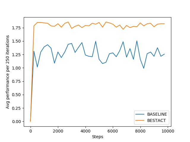
Under this policy, the agent behaves randomly all the time. It doesn't provide any significant learning but might be used as baseline to compare other RL policy learning approaches. For an instance, if it runs for 10000 iterations, it genrates graph something like this: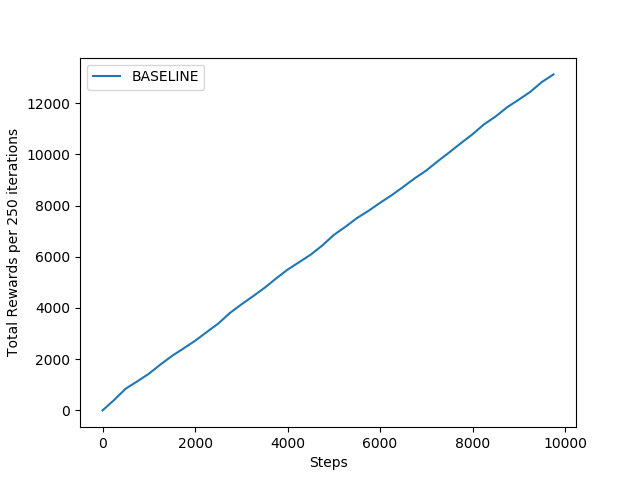
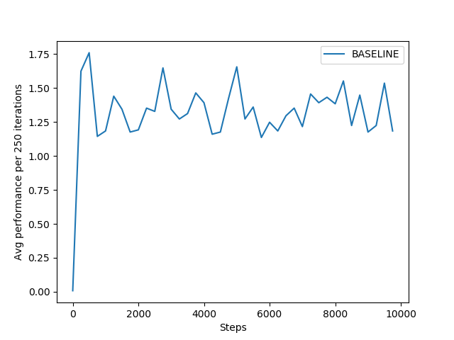
Left figure explains that total reward grows linearly with the number of iterations. Performancewise, the agent receives average rewards only upto 1.75 at maximum as per the right figure. This signifies ineffeciency of the the policy learning for the agent to achieve the desired goal. It can be used as baseline, the model delivers the performance below it, shall be dropped without any second thought.
BestAct Policy
This policy always selects best action no matter what and adds the obtained reward into the Q-Table. If it finds the Q-value of all the actions are same, it chooses an action randomly. This is the crux of this policy. It has some serious limitations.
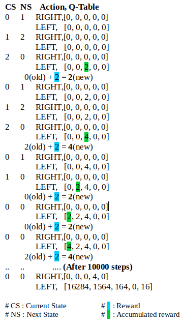
Initial 10 iteration and last of 10000 iterations are shown above for this policy. Based on the reward model, the number of agent moves towards first box is far more than the number of times it reaches to last box. This is because, the second row of the Q-Table has higher values, means agent moves mostly to left if trained by BestAct policy. Agent, get stuck on first box, because of this, the first value of second row is very high than any other element in the Q-Table.
This policy has the similar problem of unable to draw correct Q-Table, as it is not considering any context (influence of current action to future states, actions).
As this policy is greedy about Q-Values, it always achieves high total-reward and average reward. than the Baseline learning. In terms of behaviour, it is almost similar to baseline system.
Q-Learning: Quantifying importance of an Action
Q-learning is about determining a function $Q(s_t,a_t)$ of two input that evaluates the action to be taken in the current state. The value function $Q$ returns an accumulated expected reward through taking the current action (and all subsequent actions) at the present state. Initially, Q-function returns some arbitrary values, but as the agent explore the environment, it deliver better and better approximations of a pair of state $s_t$ and action $a_t$. The formula for the estimation of $Q$ is below sourced from Wikipedia:
This function tells the behind story how the concept of temporal difference is used in the estimation of new Q-values. $[r_{t+1}+\gamma\max_{a}Q(s_{t+1},a)-Q(s_t,a_t)]$ calculates the temporal difference between current Q-value and esitmated reward for next future action. $\alpha$ defines rate of learning, if its very high, it will cross the optimal and if its very low, it will take long time to reach there. $\gamma$ is discount that decides the weigh of future expected action value. Thus both defines and able to tweak the behavior of the learning algorithm.
Let's see how our agent performs and fills the Q-table through learning phase. The strategy would followed:
- Select most lucrative action.
- Sometimes actions are also chosen randomly.
- If all action values are zero, select a radom a action.
- Start with 100% radom actions(exploration) and move to 0% (exploitation)
-
Use discount
$\gamma$= 0.95 -
Use learning rate
$\alpha$= 0.1
Let's see our Agent in action!
Rate of stochasticity (exploration rate) has to be lowered down towards the end. Because, the best way to reach an optimal policy is to first explore aggressively and then move more and more convservatism. All ML follows the same mechanism.
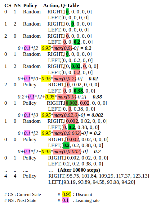
If you look in the above figure for first 10 iterations, agent decides to take action randomly many times. Its because of mainly two reasons. First, selecting actions randomly, provide agent the opportunity to explore the non-visited scenarios, which is necessary at the starting. Second, since our strategy is greedy, our agent may stuck in local optimum, not finding the optimal policy.
If you observe, first row (RIGHT) values are higher than the bottom one (LEFT), this shows the overall behaviour of the agent obtained through a number interactions. One more thing worth noting here is that how highest reward value achieved at the last tile, starts to "leak" from right to left (See the first row of Q-Table). This is the core of reinforcement learning, which allows the agent to "look into the future" and decide to take suitable action.
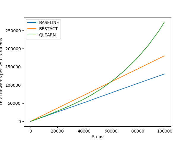
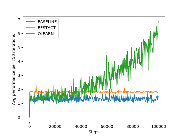
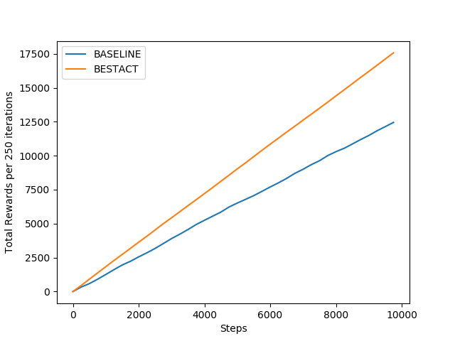
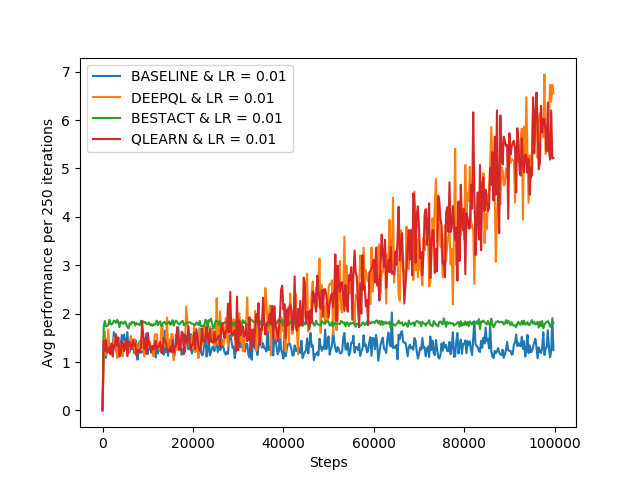
Above figures show the comparison of Q-Learning with other policies learning approaches discussed above. Though this approach is slower to converge, but achieves highest reward at the end.
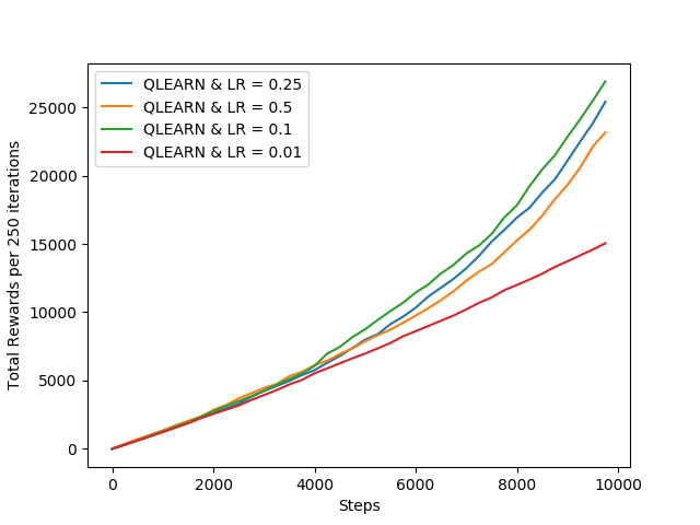
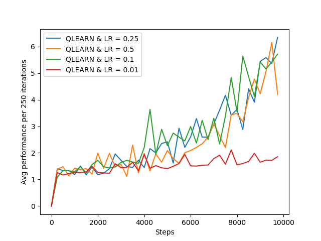
Its clear from the above figure that increase learning rate beyond 0.1 value doesn't help the agent to improve.
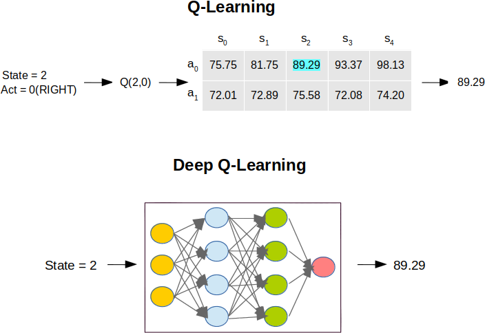
In this part, we will dive into understanding the usage of Deep Leanrnig to shift our Q-learning approach from Q-table to a deep neural net. Till now, we have seen the basics of Q-Learning in comparison with the Random Policy and BestAct policy.
Q-Learning has done its task tremendously of generating the action policy table to guide the agent, how to behave. But it suffers from the scaling limited only for certain number of states and actions. If you look up the the table takes of size in the above example, it is stateXactions as 5x2=10. What if, suppose $state=10,000$ and $action=1000$ set up the environment for the agent, the size of the table would reach to the value $10^7$ and makes the things out of control. First, the memory requirement will shoot up and then the number states to be explored for constructing "perfect Q-Table" would grow exponentially.
Here, the concept of approximation in Reinforcement learning comes to rescue the agent. Take an example of video streaming, where to communicate 1080p HD(High Definition) video at 60 frames per second would require 6GB of bandwidth of communication channel (see this link). But, when video is compressed with an lossy approach without loosing much information necessary for human visual perception, communication medium can be approximated to $1/10000th$ of its original size.
Similarly in deep Q-learning, a neural network model is used to approximate the values of Q-Table. The state being explored is given as input to the network and Q-values of all possible actions are generated as output. An easy example for comparing both is illustrated in the figure below:
Let's set the background for reinforcement learning using Deep Q-learning networks (DQNs). It follows the following steps:
-
All the past user experiences are supposed to be prestored up in memory for the training, a user experience is a list of current state, action, reward and new state.
$$Single Experience = (current ctate, action, reward, next state)$$ - The output of network is the approximate Q-values of all the possible action. Max of them will be chosen by the agent to perform at a particular state.
-
During the training, loss function is mean squared error between the predicted $\max_{a} Q(a)$ and target value $[r_{t+1}+\gamma\max_{a}Q(s_{t+1},a)]$. Let's us see why this is true. Learning rate $\alpha$ is not required as it has built-in parameter for it, instead it passed to "GradientDescentOptimizer" during the training. On removing the $\alpha$, two $Q(s,a)$ terms will also be removed. The remaining term will serve as the target value for the neural network.
$$ Q(s_t,a_t) \leftarrow [r_{t+1}+ \gamma\max_{a}Q(s_{t+1},a)] $$
Its smelling like regression is being cooked somwhere. You are not wrong, supervised learning comes here to help Reinforcement learning. The mentioned loss function estimates the error between Q-value (predicted by neural network) and target value (estimated by the above formula) which creates the basis for training regression model.
Let's see the implementation part and compare it with all the reinforcement learning approaches seen till now.
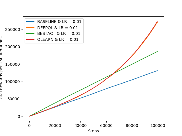
The performance of DQL varies significantly on the given value of learning rate. If learning rate is set to value 0.01, DQL perfectly get close to Q-Learning as shown in the above graph. But on other values very poor value. It is evident in the following graphs on generated on three values of LR={0.001,0.01 and 0.1}.
This is because, the simulator is not defined by all subtleties, reward mechanism is very coarse. But DNN approaches work as desired for more complex type of problem. Often, machine learning approaches work perfectly for such simple scenarios.
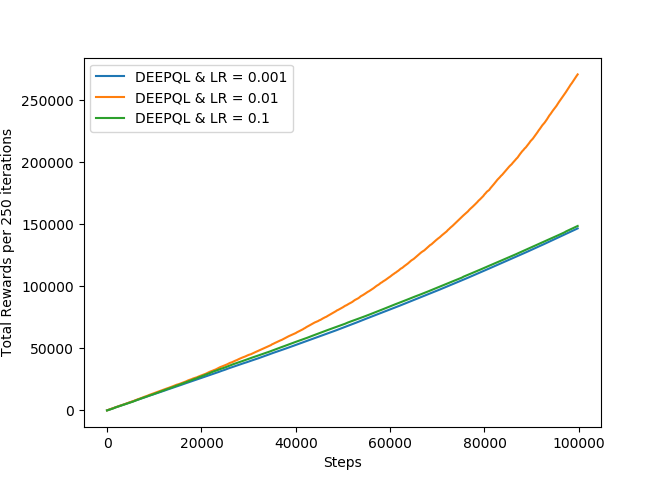
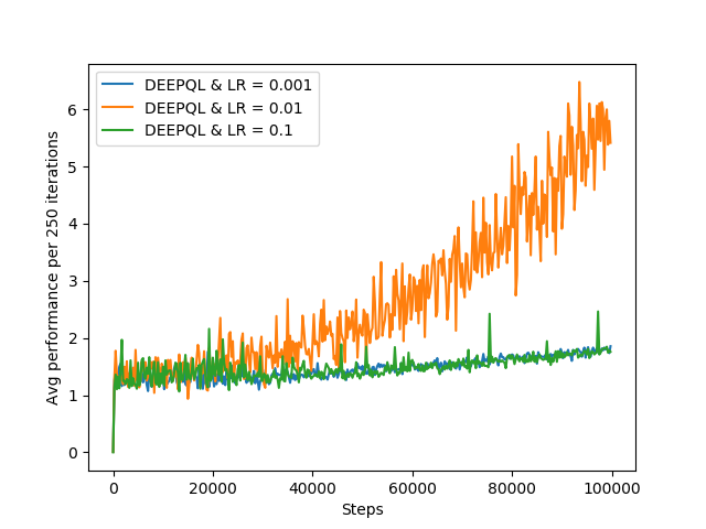
The graphs shows the effect on the change of learning rate in training Deep Learning model. When the value of LR is 0.01, it delivers its best results.
Concluding the article, we have learned the basic Reinforcement Learning models scaling from very basic Random Policy to vert complex Deep Learning. We have also seen how Q-Table is replaced with an approximated Deep Learning model as regression between state and its target value (for choosing an action). Now, we all setup to apply all these models to solve more complicated scenarious of real world problems.