Gaussian Processes (GP): Mysteries Uncovered

This post is scribbled to explore the mysteries of Gaussian Processes (GP). Initially, it provides an overview GP followed by a simple experimental analysis. Prerequisite to this post is that one should have basic knowledge of probability and machine learning (ML). Beforehand, it is important to look at Carl Rasmussen and Christopher Williams’s renowned textbook Gaussian Processes for Machine Learning as a reference.

Before going in deep with the usage of Gaussian Processes (GP), brush-up the basics of the simple linear regression. As we know that in simple linear regression, there is a dependent variable $y$ which is supposed to be modeled as a function of an independent variable $x$ like $y=f(x)+\epsilon$ where $\epsilon$ is the irreducible error. To solve this simple linear function $f$, we need to find parameters $\theta_0$ and $\theta_1$ originally representing the intercept and slope of the line respectively as in $y=\theta_0+\theta_1x$. Bayesian linear regression, a probabilistic approach, also solves a problem by finding a distribution over parameters keep updating on new data point. In contrast, GP is a non-parametric approach, which attempts to estimate a distribution over a number of possible functions $f(x)$ in cosistent with the given data points. In similar to all Bayesian methods, it starts with some prior distribution and keep updating it as data points available to training, and results as posterior distribution over all functions.

To justify the limitation of linear regression to fit a non linear data look at the following two images:

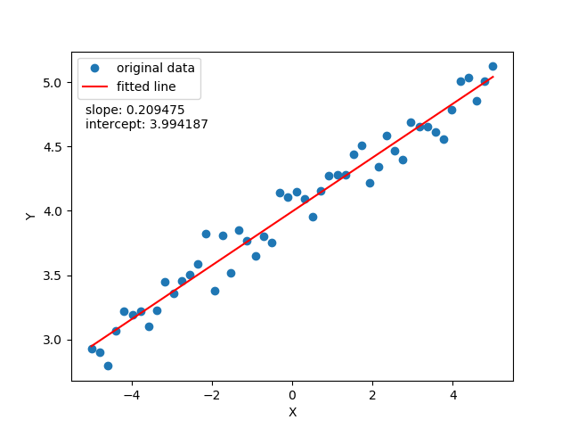
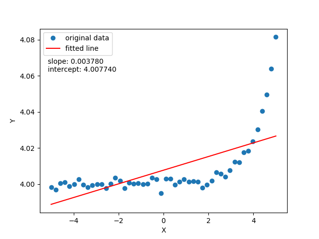
The observation is, this linear regression isn't adequate to fit non-linearly distributed data. To overcome, you'd like to fit the data with a curved line function: means in place of just 2 parameters function $\hat{y} = \theta_0$ + $\theta_1x$, a quadratic function $\hat{y} = \theta_0$ + $\theta_1x + \theta_1x^2$ would work better. But there is a catch, you would always not know the number parameters required? We want to know all possible functions with as many as parameters required to fit our data. Hence it defines the non-parametric property which doesn't suggest that there aren't parameters but there are infinitely many parameters.

Now a function need to be chosen that we want to model with GP. Let's stick a function of specific domain: $x$ values varies from -5 to 5, mean of the samples is, say 0. Consider function is not too wiggly i.e. Chebfun. Covariance matrix is a measure of smoothness of a function based on the property that near-by data points in the input space will generate output values that are also close. So finally a Gaussian Process is defined by this covariance matrix with the mean function to generate (posterior) expected value of $f(x)$. A GP is beautifully explained by Kevin Murphy in his book Machine Learning: A Probabilistic Perspective:

A GP defines a prior over functions, which can be converted into a posterior over functions once we have seen some data. Although it might seem difficult to represent a distrubtion over a function, it turns out that we only need to be able to define a distribution over the function’s values at a finite, but arbitrary, set of points, say \( x_1,\dots,x_N \). A GP assumes that \( p(f(x_1),\dots,f(x_N)) \) is jointly Gaussian, with some mean $ \mu(x) $ and covariance $ \sum(x) $ given by $ \sum_{ij} = k(x_i, x_j) $, where k is a positive definite kernel function. The key idea is that if \( x_i \) and \( x_j\) are deemed by the kernel to be similar, then we expect the output of the function at those points to be similar, too.

Source: Wikipedia

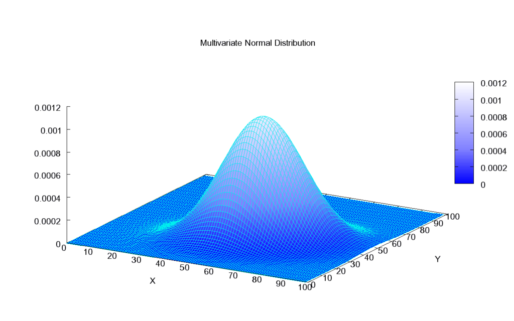
Mutlivariate Gaussian Distribution is truly modeled by GPs. In general, covariance matrix determines the shape of bell as shown in above figure. By observing the bell from the top, it looks like a perfect circle which means axis $X$ and $Y$ are independent of each other, accordingly their covariance is 0. For two independent normal distributed variables, the covariance matrix would look like $ \Sigma = \begin{bmatrix} 1 & 0\\ 0 & 1 \end{bmatrix} $.

We can represent the joint probability distribution of two variable $x_1$ and $x_2$:

Using this joint probability distribution, it is now possible to estimate the conditional probability of one variable over another.

For the sake of clear understanding, let's revise what we have seen till now. We initilised with some data points $x$ with their known outcome $f(x)$ (denoted above as $f$). Additionally, there are also some data points with unknown output values $x_*$ for which we are trying to estimate $f(x_*)$ (denoted above as $f^*$). This leads to define the final model of regression as probability distribution $p(f_* | ,x,f,x_*)$ assuming that $f$ and $f_*$ are jointly Gaussian distributed as shown earlier. Suppose, mean $\mu_*$ and covariance $\Sigma_*$ are the parameter of that joint distribution then Gaussian Regression can be defined as:

Note that this learned conditional distribution can sample as many samples we want. But before that we need to apply a trick here. As for a univariate distribution $f \sim \mathcal{N}(\mu, \sigma^2)$, you can easily express it using standard normals i.e. $f \sim \mu + \sigma(\mathcal{N}(0,1))$ but it's not that straight forward in the case of Multivariate Gaussian. But there is trick which does express this equivalently in the terms of standard normals: $f_* \sim \mu + L(\mathcal{N}(0,I))$. Here, $L$ is the square root of our covariance matrix estimated using Cholesky Decomposition shown as $LL^T = \Sigma_*$.

Let's now understand it with the code which has been borrowed from Nando de Freitas’ UBC Machine Learning lectures and with some part of linear algebra. First, we consider a test data vector Xtest consists of 50 evenly spaced data points between -5 and 5. Squared Exponential kernel $exp(-\lambda||X_i-X_j||^2)$ is used as a kernel function for estimating covariance as similarity between two data points, in order to tune the parameters. Then 5 element training vector {-4, -3, -2, -1, 1} is taken for training the joint gaussian distribution. And the actual function generating the $y$ of each training point, unknown to our model, is the $sin$function.

Firstly, covariance matrix of training K_ss=kernel(Xtrain,Xtrain) and testing K=kernel(Xtest,Xtest) denoted above as $K_{**}$ and $K$, are estimated via Squared Exponential kernel function. Then Cholesky decompostion is applied on the training data to obtain the sqaure-root matrix $L$ of its covariance $LL^T = K$ which will help the gaussian distribution to be represented through standard normals. Covariance between testing and training (denoted above as$K_*$) is also estimated with applying the similar kernel function K_s = kernel(Xtrain, Xtest). Now our goal is to estimate the mean and standard deviation of the jointly distributed gaussian of Xtrain and Xtest for generating the posteriors.

Code line Lk = np.linalg.solve(L, K_s); in the above program calculates $L^{-1}K_*$. Dot product $(L^{-1}K_*)^TL^{-1}f_* = K_*^TK^{-1}f_*$ gives the mean of the joint Gaussian. Likewise, code line s2 = np.diag(K_ss) - np.sum(Lk**2, axis=0); calculates the square of standard deviation. It can be expressed in terms of linear algebra as $K_{**} - (L^{-1}K_*)^T(L^{-1}K_*)$ or $K_{**} - (K_*^TK^{-1}K_*)$.

# This code implements a simple GP regression using Cholesky Decomposition.
# It assumes a zero mean GP Prior.
import numpy as np
import matplotlib.pyplot as pl


f = lambda x: np.sin(0.9*x).flatten()
#f = lambda x: (0.25*(x**2)).flatten()

# Test data
n = 50
Xtest = np.linspace(-5, 5, n).reshape(-1,1)

Xtrain = np.array([-4, -3, -2, -1, 1]).reshape(5,1)
ytrain = np.sin(0.9*Xtrain)

# Define the kernel function => Squared exponential = exp(-0.5*(1/param)*(a-b)^2)
def kernel(a,b,param):
    sqdist = np.sum(a**2,1).reshape(-1,1) + np.sum(b**2,1)-2*np.dot(a,b.T)
    return np.exp(-.5*(1/param)*sqdist)

param = 0.1
# Apply the kernel function to testing points to get K_**
K_ss = kernel(Xtest, Xtest, param)
# Apply the kernel function to our training points to get K
K = kernel(Xtrain, Xtrain, param)
# Apply the Cholesky function as for getting (K=LL^T)
L = np.linalg.cholesky(K + 0.00005*np.eye(len(Xtrain)))

# Compute the mean at our test points.

# Apply the kernel function to our training points to get K_*
K_s = kernel(Xtrain, Xtest, param)
# Solving L*x = K_* => x = (L^-1*K_*)
Lk = np.linalg.solve(L, K_s)
# Mean is calculated as => (L^-1*K_*)^T * L^-1f = K_*^T K^-1 f
mu = np.dot(Lk.T, np.linalg.solve(L, ytrain)).reshape((n,))

# Standard deviation sqrt of variance estimated as => K_** - (L^-1*K_*)^T * (L^-1*K_*) = K_** - K_*^T K^-1 * K_*
s2 = np.diag(K_ss) - np.sum(Lk**2, axis=0)
stdv = np.sqrt(s2)
# Draw samples from the posterior at our test points.
L = np.linalg.cholesky(K_ss + 1e-6*np.eye(n) - np.dot(Lk.T, Lk))
f_post = mu.reshape(-1,1) + np.dot(L, np.random.normal(size=(n,4)))

# draw samples from the prior at our test points.
L = np.linalg.cholesky(K_ss + 1e-6*np.eye(n))
f_prior = np.dot(L, np.random.normal(size=(n,5)))
pl.figure(1)
pl.clf()
pl.plot(Xtest, f_prior)
pl.title('Ten samples from the GP prior')
pl.axis([-5, 5, -3, 3])
pl.savefig('prior.png', bbox_inches='tight')

# draw samples from the posterior at our test points.
L = np.linalg.cholesky(K_ss + 1e-6*np.eye(n) - np.dot(Lk.T, Lk))
f_post = mu.reshape(-1,1) + np.dot(L, np.random.normal(size=(n,5)))
pl.figure(2)
pl.clf()
pl.plot(Xtest, f_post)
pl.title('Ten samples from the GP posterior')
pl.axis([-5, 5, -3, 3])
pl.savefig('post.png', bbox_inches='tight')

# draw stdev

pl.plot(Xtrain, ytrain, 'bs', ms=8)
pl.plot(Xtest, f(Xtest), 'b-')
pl.gca().fill_between(Xtest.flat, mu-3*stdv, mu+3*stdv, color="#dddddd")
pl.plot(Xtest, mu, 'r--', lw=2)
pl.title('Mean predictions plus 3 st.deviations')
pl.axis([-5, 5, -3, 3])
pl.savefig('predictive.png', bbox_inches='tight')

pl.show()

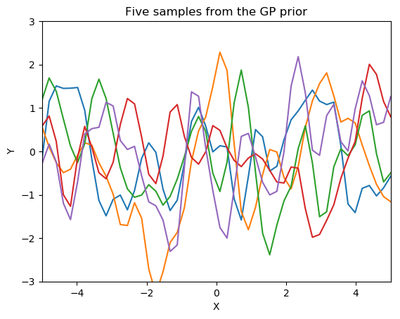
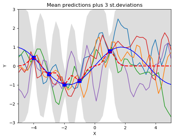
See how the training data (the blue squars in the right graph) rule over the set of the possible function being generated through the posterior of GP. All function pass through all the training points. Left graph show the distribution of samples before training. The red dotten line and gray shaded area show the mean and standard deviation respectively of the joint gaussian distribution. The region where data is unavailable for training the standard deviation is very high. Means for better trained Gaussian Regression a significant amount of training data should be available.

This post has presented a very simple picture of Gaussian Processes highlighting the important aspects of GP modelling as a non-parametric and probablistic method. This post is just a scratch at the surface of all possible wonders which could be done by GP in the field of Machine Learning and Artifical Intelligence!